Branching Dataflow Gen2 Outputs to Multiple Destinations: Writing Transformed Data to a Lakehouse Table and a Warehouse Simultaneously
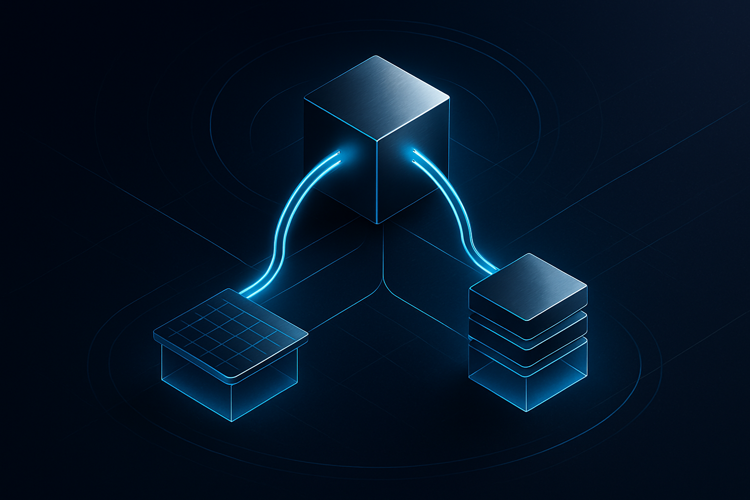
Dataflow Gen2 lets you attach multiple output destinations to a single query — run your transformation once and write results to both a Fabric Lakehouse table and a Warehouse table simultaneously. This lesson teaches you the complete pattern: from Power Query transformation to dual-destination configuration, data type gotchas, and production-ready pipeline orchestration.
⚡ Practitioner22 min readSep 22, 2026Updated Sep 22, 2026
On this page
Branching Dataflow Gen2 Outputs to Multiple Destinations: Writing Transformed Data to a Lakehouse Table and a Warehouse Simultaneously
Introduction
Here's a scenario that comes up constantly in real-world Fabric implementations: your analytics team wants to query transformed sales data from a Fabric Warehouse using clean T-SQL and stored procedures, while your data science team wants that same cleaned dataset landing in a Lakehouse where they can run Spark notebooks against it. You've already written the transformation logic once in Dataflow Gen2 — the last thing you want to do is maintain two separate dataflows with identical Power Query steps just to feed two different destinations.
The good news is that Dataflow Gen2 has a feature purpose-built for exactly this problem: output destinations. Unlike the original Dataflow Gen1 where a query had exactly one place to go, Gen2 lets you attach multiple output destinations to the same query. That means your transformation runs once, and the results get written simultaneously to as many Fabric items as you need. One cleaned dataset, multiple consumers, zero duplication of logic.
By the end of this lesson, you'll know how to configure a single Dataflow Gen2 query to write its output to both a Lakehouse managed table and a Warehouse table at the same time. You'll understand how Fabric physically executes that dual write, where the gotchas are, and how to make this pattern production-ready inside a data pipeline.
What you'll learn:
- How Dataflow Gen2 output destinations differ from the single-sink model of Gen1 and classic Power Query
- How to configure a Lakehouse table destination and a Warehouse table destination on the same query
- How schema mapping, update methods, and data type handling work for each destination type
- How to wrap a multi-destination dataflow in a Data Pipeline for orchestration and scheduling
- How to troubleshoot the most common failures specific to branched outputs
Prerequisites
This lesson assumes you're already comfortable with the basics of Dataflow Gen2 and Power Query transformations. If you're newer to the tool, spend some time with Ingesting Data with Dataflow Gen2: Power Query Skills in Microsoft Fabric before continuing — we'll be moving fast through the Power Query side and spending our energy on the output configuration.
You should also have:
- A Fabric workspace with at least Contributor rights (an F2 or trial capacity works fine — see Fabric Capacities and Workspaces: F SKUs, Trials, and Setting Up Your First Workspace if you need to set one up)
- An existing Lakehouse with the Tables section available
- An existing Fabric Warehouse
- A source dataset to work with — we'll use a realistic sales orders example throughout
Understanding How Multi-Destination Outputs Actually Work
Before you click a single button, let's get the mental model right — because if you misunderstand what Fabric is doing under the hood, you'll make configuration mistakes that are hard to debug.
When you add an output destination to a Dataflow Gen2 query, you are not adding a second copy of the dataflow. You are telling the Fabric backend that after the query finishes evaluating, it should write the result set to an additional location. Internally, Dataflow Gen2 uses a staging area in OneLake — a temporary location where your transformed data lands first before being pushed to each configured destination.
This staging step is what makes multi-destination possible. The query evaluates once, the result set materializes in staging, and then separate write operations fan out from that staging area to each destination. Think of it like a mail sorting facility: one inbound truck (your query result), multiple outbound routes (your destinations).
Key insight
The staging area in OneLake is what decouples your transformation logic from your output destinations. It's also why you need a Fabric capacity — the staging storage is provisioned automatically and doesn't require any configuration from you, but it does require the Fabric compute layer.
There's an important implication here for data consistency. Because each destination write is a separate operation, they don't happen in a single atomic transaction. In the vast majority of cases this is fine — both writes will succeed or the dataflow will fail and retry — but it's worth knowing that if the dataflow fails midway through writing to the second destination, you could briefly have fresh data in one location and stale data in the other. We'll discuss how to handle this in the pipeline orchestration section.
Setting Up the Scenario: A Sales Orders Transformation
Let's work with something concrete. Imagine you're pulling daily sales order data from an Azure SQL Database. The raw data has messy column names, some inconsistent casing in product category names, and a calculated margin column that doesn't exist in the source. After transformation, the cleaned result needs to:
- Land in a Lakehouse table called
gold_sales_orders, used by the Direct Lake semantic model powering executive dashboards - Land in a Warehouse table called
dbo.fact_sales_orders, used by the BI team for T-SQL-based reporting and ad hoc queries
Same data, two consumers, one transformation. Let's build it.
Step 1: Create a New Dataflow Gen2
In your Fabric workspace, select New and then Dataflow Gen2. You'll land in the Power Query Online editor — a familiar interface if you've used Power Query in Excel or Power BI Desktop.
Connect to your source. For this example, we're connecting to Azure SQL Database using the SQL Server connector. Enter your server name, database name, and credentials. Navigate to the SalesOrders table and select it.
Your raw query will look something like this in Power Query M (you can view it by going to Home > Advanced Editor):
let
    Source = Sql.Database("myserver.database.windows.net", "SalesDB"),
    SalesOrders = Source{[Schema="dbo", Item="SalesOrders"]}[Data]
in
    SalesOrders
Step 2: Apply Your Transformations
Now apply the transformation steps that produce the clean, analysis-ready dataset. In the Power Query editor, you'd do this through the UI, but here's the full M script so you can see exactly what's happening:
let
    Source = Sql.Database("myserver.database.windows.net", "SalesDB"),
    SalesOrders = Source{[Schema="dbo", Item="SalesOrders"]}[Data],

    // Rename columns to clean snake_case names
    RenamedColumns = Table.RenameColumns(SalesOrders, {
        {"OrderID", "order_id"},
        {"CustID", "customer_id"},
        {"OrderDate", "order_date"},
        {"ShipDate", "ship_date"},
        {"ProdCategory", "product_category"},
        {"ProdName", "product_name"},
        {"UnitPrice", "unit_price"},
        {"Qty", "quantity"},
        {"Discount", "discount_pct"},
        {"Revenue", "revenue"},
        {"COGS", "cost_of_goods_sold"}
    }),

    // Normalize product category casing
    NormalizedCategory = Table.TransformColumns(
        RenamedColumns,
        {{"product_category", Text.Proper, type text}}
    ),

    // Add calculated margin column
    AddedMargin = Table.AddColumn(
        NormalizedCategory,
        "gross_margin",
        each [revenue] - [cost_of_goods_sold],
        type number
    ),

    // Filter out test orders (order_id starts with "TEST-")
    FilteredOrders = Table.SelectRows(
        AddedMargin,
        each not Text.StartsWith([order_id], "TEST-")
    ),

    // Set correct data types explicitly
    TypedTable = Table.TransformColumnTypes(FilteredOrders, {
        {"order_id", type text},
        {"customer_id", type text},
        {"order_date", type date},
        {"ship_date", type date},
        {"product_category", type text},
        {"product_name", type text},
        {"unit_price", type number},
        {"quantity", type Int64.Type},
        {"discount_pct", type number},
        {"revenue", type number},
        {"cost_of_goods_sold", type number},
        {"gross_margin", type number}
    })
in
    TypedTable
Notice that the last step explicitly sets data types. This is not optional when you're writing to multiple destinations — it's critical. Each destination enforces its own schema, and letting Power Query infer types is an invitation for silent mismatches.
Warning
If you don't explicitly define column types in your Power Query steps, Dataflow Gen2 will infer them from the first batch of data it sees. This works until a batch comes through with a null in a column it thought was Int64, or a value that looks like a date but is actually a string. Always set your types explicitly before configuring output destinations.
Configuring the First Destination: Lakehouse Table
With your query producing clean, correctly-typed data, it's time to add destinations. In the Dataflow Gen2 editor, look at the bottom of the screen — you'll see a panel called Query settings on the right, and at the bottom of the canvas you'll find the Add data destination button. In some layouts, you'll see it as a "+" icon in the lower right of the query card itself.
Click Add data destination and select Lakehouse from the list of options.
Connecting to Your Lakehouse
A connection dialog will appear. If you haven't connected to this Lakehouse from a dataflow before, you'll need to establish the connection. Select your workspace from the dropdown, then select your Lakehouse item. You'll then specify:
- Root folder: Tables (this is where managed Delta tables live — using the Files section here would write raw files, not queryable tables)
- Table name:
gold_sales_orders
If the table doesn't exist yet, Fabric will create it. If it does exist, you'll get to choose how to handle the existing data.
Choosing an Update Method
This is one of the most consequential decisions in the destination configuration, and the one most people get wrong the first time.
You have two options:
Append: New rows are added to the existing table each time the dataflow runs. Use this when your query returns only new records (i.e., you've already filtered to today's data or new records since last run).
Replace: The table is truncated and all rows from the current query result are written fresh. Use this when your query always returns the full current state of the data.
For our sales orders scenario, let's assume we're running an incremental pattern where the dataflow pulls all orders from the past 30 days and we want the table to always reflect that rolling window. That means Replace is the right choice — we don't want to accumulate 30-day snapshots on top of each other.
Tip
If you need a true incremental merge (upsert based on a key), Dataflow Gen2's built-in update methods won't do it natively at the destination level. For that pattern, consider landing to the Lakehouse with Replace and then running a separate Spark notebook to handle the merge, or use a pipeline with a Copy Activity into a staging table followed by a T-SQL MERGE.
Schema Mapping
After selecting the update method, you'll see the Column mapping screen. This shows the columns coming from your query on the left and the destination columns on the right.
If the table is new, Fabric proposes to auto-create the schema based on your query's column types — accept this and verify each type. If you're mapping to an existing table, carefully check that each source column aligns to the correct destination column. A common mistake here is leaving columns unmapped because of a name mismatch between your query output and an existing table.
For gold_sales_orders, our new table, the auto-mapping should be clean since we explicitly typed everything in the query. Confirm and save.
Configuring the Second Destination: Warehouse Table
Now for the second destination. With your query still selected in the canvas, click Add data destination again — yes, the same button, on the same query. This time select Warehouse.
Connecting to Your Warehouse
The connection flow is similar to the Lakehouse. Select your workspace, then your Warehouse item. You'll then specify the schema and table name:
- Schema:
dbo - Table name:
fact_sales_orders
Note
Unlike Lakehouse destinations where you're working with Delta tables managed in OneLake, a Warehouse destination writes to tables managed by the Warehouse's SQL engine. If you want to understand the architectural differences between these two storage types and when each one makes sense, Fabric Lakehouse vs Warehouse: Choosing the Right Store for Your Workload covers that decision in depth.
Update Method for the Warehouse Destination
The same Append vs. Replace choice applies here, and you should make the same decision you made for the Lakehouse — in our case, Replace. The key thing to understand is that each destination can have a different update method.
This is actually quite powerful. You could, for example:
- Write to the Lakehouse with Append to build a historical archive with every row ever processed
- Write to the Warehouse with Replace to maintain a current-state table for BI consumption
The same query result fans out to both, but each destination handles the data according to its own write mode.
Data Type Considerations for Warehouse Destinations
Here's where practitioners get caught. Fabric Warehouse tables use T-SQL data types, and the mapping from Power Query types to T-SQL types isn't always intuitive:
| Power Query Type | T-SQL Type in Warehouse |
|---|---|
type text |
varchar(8000) |
type number (decimal) |
decimal(18,0) — watch the precision! |
Int64.Type |
bigint |
type date |
date |
type datetime |
datetime2(7) |
type logical |
bit |
The most common pain point is type number mapping to decimal(18,0), which silently truncates your decimal places. If unit_price is 24.99 and lands as 25 in your Warehouse table, this is why.
The fix: pre-create the Warehouse table with the exact types you want before configuring the destination. When Dataflow Gen2 finds an existing table, it maps to the existing column types rather than trying to create them. Open your Warehouse and run:
CREATE TABLE dbo.fact_sales_orders (
    order_id        VARCHAR(50)       NOT NULL,
    customer_id     VARCHAR(50)       NOT NULL,
    order_date      DATE              NOT NULL,
    ship_date       DATE              NULL,
    product_category VARCHAR(100)     NOT NULL,
    product_name    VARCHAR(200)      NOT NULL,
    unit_price      DECIMAL(10, 2)    NOT NULL,
    quantity        INT               NOT NULL,
    discount_pct    DECIMAL(5, 4)     NULL,
    revenue         DECIMAL(18, 2)    NOT NULL,
    cost_of_goods_sold DECIMAL(18, 2) NOT NULL,
    gross_margin    DECIMAL(18, 2)    NOT NULL
);
Now when you configure the Warehouse destination and Fabric sees this existing table, it will respect your DECIMAL(10,2) definition rather than defaulting to DECIMAL(18,0). This is the most reliable way to get precise type control for Warehouse destinations.
Warning
If you let Dataflow Gen2 auto-create the Warehouse table and your type number columns get created as decimal(18,0), you won't see an error — the data will just silently lose its decimal precision. Always pre-create Warehouse tables with explicit types when precision matters, which for financial data is essentially always.
Verifying Your Dual-Destination Configuration
Before you publish and run, take a moment to verify both destinations are correctly attached. In the Power Query canvas, your query card should show two destination indicators — typically rendered as small icons or badges at the bottom of the query card, one for the Lakehouse and one for the Warehouse.
You can click on each destination indicator to open the configuration and double-check:
- The correct workspace and item are selected
- The table name is correct
- The update method matches your intent
- The column mapping shows all columns correctly aligned
If a column appears unmapped (greyed out or flagged), stop and resolve it before publishing. An unmapped column means that column will be silently dropped during the write — no error, just missing data.
Publishing and Running
Click Publish in the top right of the Dataflow Gen2 editor. Publishing saves and triggers the dataflow to run immediately. You'll see a notification that the dataflow is refreshing.
To monitor the run, navigate to the Monitoring Hub in your workspace. You'll see the dataflow appear with its current status. A successful run for a multi-destination dataflow shows one overall status — Fabric handles both writes as part of the same dataflow execution.
Once complete:
- Open your Lakehouse and navigate to Tables — you should see
gold_sales_orderswith data - Open your Warehouse and query
dbo.fact_sales_orders:
SELECT TOP 10
    order_id,
    order_date,
    product_category,
    revenue,
    gross_margin
FROM dbo.fact_sales_orders
ORDER BY order_date DESC;
Both should show identical row counts and data.
Wrapping the Dataflow in a Data Pipeline
Running a multi-destination dataflow on a manual publish schedule is fine for development, but in production you want orchestrated, scheduled execution with retry logic and alerting. That means wrapping it in a Data Pipeline.
Why Pipeline Orchestration Matters Here
Remember the data consistency concern we flagged earlier — the two destination writes are not atomic. If your dataflow succeeds in writing to the Lakehouse but fails midway through writing to the Warehouse, you'll have an inconsistency until the next successful run.
A pipeline gives you:
- Retry logic at the activity level — if the dataflow fails, the pipeline can retry automatically
- Dependency chaining — you can run validation queries after the dataflow completes to confirm both destinations have expected row counts
- Alerting — email notifications when the pipeline fails, before your downstream consumers notice
Building the Pipeline
Create a new Data Pipeline in your workspace. Add a Dataflow activity — this is the activity type for invoking a Dataflow Gen2. Configure it to point to your newly published dataflow.
After the Dataflow activity, add two Script activities (or Lookup activities against the SQL Analytics Endpoint / Warehouse) to run validation queries. Connect them in parallel off the success path of the Dataflow activity:
Validation Query for Lakehouse (via the SQL Analytics Endpoint):
SELECT COUNT(*) AS row_count
FROM gold_sales_orders
WHERE order_date >= CAST(DATEADD(day, -30, GETDATE()) AS DATE);
Validation Query for Warehouse:
SELECT COUNT(*) AS row_count
FROM dbo.fact_sales_orders
WHERE order_date >= CAST(DATEADD(day, -30, GETDATE()) AS DATE);
Add a final Script or Set Variable activity that compares the two counts. If they differ by more than a small tolerance (accounting for any timing differences), trigger a pipeline failure or send an alert.
Tip
For the Lakehouse validation query, use the SQL Analytics Endpoint connection string, which gives you T-SQL access to your Lakehouse Delta tables without needing a Warehouse. This pattern is covered in detail in Querying Lakehouse Data with the SQL Analytics Endpoint: Writing T-SQL Against Delta Tables Without a Warehouse.
Scheduling
Set your pipeline schedule based on how frequently your source data updates. For daily sales data, a morning run (say 6:00 AM) gives the overnight batch time to complete before the pipeline kicks off. Configure the schedule on the pipeline, not the dataflow itself — when a pipeline owns the execution, you get centralized monitoring and control.
Hands-On Exercise
Let's put everything together in a structured exercise you can complete in your own Fabric environment.
Scenario
You work for a retail company that processes e-commerce orders. Your source is a SQL table called raw_orders in an Azure SQL Database (or you can simulate this with any table you have access to). The business needs:
- A Lakehouse table
gold_orders_summaryfor Direct Lake reporting - A Warehouse table
dbo.dim_orders_reportingfor the BI team's T-SQL reports
Steps
Step 1: Prepare your Warehouse table
Open your Fabric Warehouse and run the following DDL to pre-create the destination table with correct types:
CREATE TABLE dbo.dim_orders_reporting (
    order_id            VARCHAR(50)     NOT NULL,
    customer_id         VARCHAR(50)     NOT NULL,
    order_date          DATE            NOT NULL,
    product_category    VARCHAR(100)    NOT NULL,
    revenue             DECIMAL(18, 2)  NOT NULL,
    gross_margin        DECIMAL(18, 2)  NOT NULL,
    margin_pct          DECIMAL(7, 4)   NULL,
    is_discounted       BIT             NOT NULL,
    load_timestamp      DATETIME2(0)    NOT NULL
);
Step 2: Build the Dataflow Gen2
Create a new Dataflow Gen2 and connect to your source table. Apply these transformations:
let
    Source = /* your source connection here */,

    // Add margin percentage
    AddedMarginPct = Table.AddColumn(
        Source,
        "margin_pct",
        each if [revenue] = 0 then null else ([revenue] - [cost_of_goods_sold]) / [revenue],
        type number
    ),

    // Add boolean discount flag
    AddedDiscountFlag = Table.AddColumn(
        AddedMarginPct,
        "is_discounted",
        each [discount_pct] > 0,
        type logical
    ),

    // Add load timestamp
    AddedTimestamp = Table.AddColumn(
        AddedDiscountFlag,
        "load_timestamp",
        each DateTimeZone.RemoveZone(DateTimeZone.LocalNow()),
        type datetime
    ),

    // Select and reorder only the columns we need
    FinalColumns = Table.SelectColumns(
        AddedTimestamp,
        {"order_id", "customer_id", "order_date", "product_category",
         "revenue", "gross_margin", "margin_pct", "is_discounted", "load_timestamp"}
    )
in
    FinalColumns
Step 3: Configure both destinations
- Add the Lakehouse destination: select your Lakehouse, set the table name to
gold_orders_summary, set update method to Replace - Add the Warehouse destination: select your Warehouse, point to
dbo.dim_orders_reporting, set update method to Replace
Step 4: Publish and verify
Publish the dataflow and wait for it to complete. Then verify:
-- In Warehouse
SELECT
    COUNT(*) AS warehouse_count,
    MIN(order_date) AS earliest_order,
    MAX(order_date) AS latest_order,
    SUM(revenue) AS total_revenue
FROM dbo.dim_orders_reporting;
Run the equivalent query against your Lakehouse via the SQL Analytics Endpoint and confirm the numbers match.
Step 5: Wrap in a pipeline
Create a Data Pipeline, add a Dataflow activity pointing to your dataflow, and set a daily schedule.
Common Mistakes & Troubleshooting
"Destination write failed" with no useful error message
This is the most common frustration. The dataflow runs, transformations complete, and then the destination write fails cryptically. Nine times out of ten, it's a data type mismatch. Go to the Monitoring Hub, open the dataflow run details, and look at the activity logs — they usually contain the specific column and type that caused the issue. Fix by either adjusting your Power Query types or altering the destination table's column definition.
One destination succeeds, the other fails
Since the two writes are separate operations, this can happen. The most common cause is a permissions issue — the dataflow's service principal or user identity has access to one item but not the other. Verify that your Fabric identity has at minimum Write access to both the Lakehouse and the Warehouse. Check item permissions from the workspace, not just workspace-level roles.
Columns are present in the query but missing in the destination table
This is the silent unmapped column problem. Go back into the dataflow editor, click on the destination indicator for the affected destination, and open the column mapping. Any column showing as unmapped will be dropped. Either map it manually or, for Warehouse destinations, add the column to the table definition first.
Dataflow times out on large datasets
By default, Dataflow Gen2 queries have a timeout. For large source tables, the query evaluation plus two writes can exceed this. Solutions:
- Push filtering further upstream — use query folding to filter at the source before data moves to the Fabric compute layer
- Implement incremental loading with watermarks so each run processes only new records rather than the full table
- For very large datasets, consider replacing the Dataflow with a Spark notebook that handles the transformation and writes directly — Transforming Data with Spark Notebooks in Microsoft Fabric: PySpark for Lakehouse Tables covers this pattern
The Lakehouse table exists but isn't recognized by the Direct Lake semantic model
This happens when the Delta table metadata isn't updated properly. After a Replace write, Direct Lake semantic models need the table's metadata to be current. In most cases, this resolves automatically, but if you're seeing stale data in reports, open the Lakehouse, navigate to the table, and use the Refresh option. You can also trigger a Delta table optimization from a notebook. The details of keeping Delta tables healthy for Direct Lake are covered in Connecting a Power BI Semantic Model to a Fabric Lakehouse in Direct Lake Mode.
Key insight
Query folding is your best friend for multi-destination dataflows. If your source supports it (SQL databases, SharePoint lists, OData feeds all do), Power Query will push as much of your transformation as possible back to the source — filtering, column selection, aggregations. This means less data travels to the Fabric staging area, transformations run faster, and your destination writes start sooner. You can verify folding is happening by right-clicking a query step and checking whether "View Native Query" is available.
Performance Implications and When to Use This Pattern
Multi-destination dataflows are powerful but not always the right tool. Here's an honest assessment of when to reach for this pattern versus alternatives.
Use multi-destination Dataflow Gen2 when:
- Your transformation logic is moderate complexity (dozens of steps, not hundreds)
- Your dataset fits comfortably in Fabric's Dataflow compute (roughly under 1-2 GB of result set)
- The two destinations need the same data (same columns, same granularity)
- You want a no-code-adjacent experience that non-engineers can maintain
Consider alternatives when:
- Your result set is large (hundreds of millions of rows) — Spark notebooks with PySpark will outperform Dataflow compute here
- You need different aggregations or granularities for each destination — at that point, use separate dataflows or separate queries within one dataflow, each with its own destination
- You need true transactional consistency across destinations — Dataflow Gen2 can't guarantee atomic writes across two items; a pipeline with compensating transactions is more appropriate
The architecture this supports best is the Gold layer of a Medallion Architecture where you have clean, business-ready data that needs to be accessible to both SQL consumers (Warehouse) and file/Spark consumers (Lakehouse). Instead of two separate ETL paths from Bronze to Gold, you have one transformation and two output paths.
Summary & Next Steps
You now know how to configure a Dataflow Gen2 query to write its results to a Lakehouse table and a Warehouse table simultaneously — and more importantly, you understand why it works the way it does (staging area, separate write operations, independent update methods) and what can go wrong (type mismatches, unmapped columns, permissions gaps, non-atomic writes).
The pattern you've built here — one transformation, multiple destinations, wrapped in a pipeline — is a production-grade pattern used in real Fabric implementations. It eliminates duplicated transformation logic, keeps your data in sync across consumer types, and integrates cleanly with the orchestration and monitoring tools Fabric provides.
Where to go next:
- If your Warehouse destination is growing complex with multiple fact and dimension tables, learn how to build a full dimensional model in Building a Fabric Data Warehouse with T-SQL: Tables, Views, and Cross-Database Queries
- If you need to make your dataflow logic reusable across environments with dynamic parameters, Parameterizing Dataflow Gen2 Queries with Pipeline Integration covers exactly that
- To promote your dataflows and pipelines from development to production workspaces, explore Fabric Git Integration and Deployment Pipelines
Microsoft Fabric Fundamentals
Previous
Creating and Managing Fabric Lakehouses with Notebooks: Reading External Files from OneLake, Writing Delta Tables, and Browsing Results in the Lakehouse Explorer
Next
Handling Schema Evolution in Fabric Lakehouse Delta Tables: Adding Columns, Merging Incompatible Schemas, and Enforcing Constraints Across Medallion Layers
Related Insights
Microsoft FabricPractitioner
Deduplicating and Cleansing Lakehouse Delta Tables with PySpark: Drop Duplicates, Fill Nulls, and Enforce Data Quality Rules Across Medallion Layers
20 min
Microsoft FabricExpert
Implementing Incremental Refresh for Direct Lake Semantic Models in Microsoft Fabric: Configuring Delta Table Partitioning, Framing Policies, and Triggering Refresh via the XMLA Endpoint
26 min
Microsoft FabricPractitioner
Orchestrating Multi-Notebook Workflows in Microsoft Fabric: Using Pipeline Notebook Activities, Activity Dependencies, and Output Variables to Chain PySpark Transformations Across Medallion Layers
20 min